###############################################################################
# The Institute for the Design of Advanced Energy Systems Integrated Platform
# Framework (IDAES IP) was produced under the DOE Institute for the
# Design of Advanced Energy Systems (IDAES).
#
# Copyright (c) 2018-2023 by the software owners: The Regents of the
# University of California, through Lawrence Berkeley National Laboratory,
# National Technology & Engineering Solutions of Sandia, LLC, Carnegie Mellon
# University, West Virginia University Research Corporation, et al.
# All rights reserved.  Please see the files COPYRIGHT.md and LICENSE.md
# for full copyright and license information.
###############################################################################

Autothermal Reformer Flowsheet Optimization with PySMO Surrogate Object

1. Introduction

This example demonstrates autothermal reformer optimization leveraging the PySMO Polynomial surrogate trainer. Other than the specific training method syntax, this workflow is identical for PySMO RBF and PySMO Kriging surrogate models. In this notebook, sampled simulation data will be used to train and validate a surrogate model. IDAES surrogate plotting tools will be utilized to visualize the surrogates on training and validation data. Once validated, integration of the surrogate into an IDAES flowsheet will be demonstrated.

2. Problem Statement

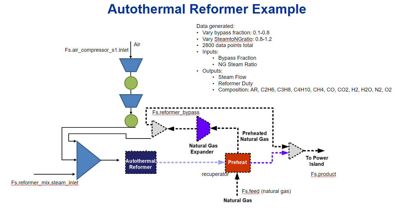
Within the context of a larger NGFC system, the autothermal reformer generates syngas from air, steam and natural gas for use in a solid-oxide fuel cell (SOFC).

2.1. Main Inputs:

• Bypass fraction (dimensionless) - split fraction of natural gas to bypass AR unit and feed directly to the power island

• NG-Steam Ratio (dimensionless) - proportion of natural relative to steam fed into AR unit operation

2.2. Main Outputs:

• Steam flowrate (kg/s) - inlet steam fed to AR unit

• Reformer duty (kW) - required energy input to AR unit

• Composition (dimensionless) - outlet mole fractions of components (Ar, C2H6, C3H8, C4H10, CH4, CO, CO2, H2, H2O, N2, O2)

from IPython.display import Image
from pathlib import Path


def datafile_path(name):
    return Path("..") / name


Image(datafile_path("AR_PFD.png"))

3. Training and Validating Surrogates

First, let’s import the required Python, Pyomo and IDAES modules:

# Import statements
import os
import numpy as np
import pandas as pd

# Import Pyomo libraries
from pyomo.environ import (
    ConcreteModel,
    SolverFactory,
    value,
    Var,
    Constraint,
    Set,
    Objective,
    maximize,
)
from pyomo.common.timing import TicTocTimer

# Import IDAES libraries
from idaes.core.surrogate.sampling.data_utils import split_training_validation
from idaes.core.surrogate.pysmo_surrogate import PysmoPolyTrainer, PysmoSurrogate
from idaes.core.surrogate.plotting.sm_plotter import (
    surrogate_scatter2D,
    surrogate_parity,
    surrogate_residual,
)
from idaes.core.surrogate.surrogate_block import SurrogateBlock
from idaes.core import FlowsheetBlock
from idaes.core.util.convergence.convergence_base import _run_ipopt_with_stats

3.1 Importing Training and Validation Datasets

In this section, we read the dataset from the CSV file located in this directory. 2800 data points were simulated from a rigorous IDAES NGFC flowsheet using a grid sampling method. For simplicity and to reduce training runtime, this example randomly selects 100 data points to use for training/validation. The data is separated using an 80/20 split into training and validation data using the IDAES split_training_validation() method.

# Import Auto-reformer training data
np.set_printoptions(precision=6, suppress=True)

csv_data = pd.read_csv(datafile_path("reformer-data.csv"))  # 2800 data points
data = csv_data.sample(n=100)  # randomly sample points for training/validation
input_data = data.iloc[:, :2]
output_data = data.iloc[:, 2:]

# Define labels, and split training and validation data
# note that PySMO requires that labels are passed as string lists
input_labels = list(input_data.columns)
output_labels = list(output_data.columns)

n_data = data[input_labels[0]].size
data_training, data_validation = split_training_validation(
    data, 0.8, seed=n_data
)  # seed=100

3.2 Training Surrogates with PySMO

IDAES builds a model class for each type of PySMO surrogate model. In this case, we will call and build the Polynomial Regression class. Regression settings can be directly passed as class arguments, as shown below. In this example, allowed basis terms span a 6th order polynomial as well as a variable product, and data is internally cross-validated using 10 iterations of 80/20 splits to ensure a robust surrogate fit. Note that PySMO uses cross-validation of training data to adjust model coefficients and ensure a more accurate fit, while we separate the validation dataset pre-training in order to visualize the surrogate fits.

Finally, after training the model we save the results and model expressions to a folder which contains a serialized JSON file. Serializing the model in this fashion enables importing a previously trained set of surrogate models into external flowsheets. This feature will be used later.

# capture long output (not required to use surrogate API)
from io import StringIO
import sys

stream = StringIO()
oldstdout = sys.stdout
sys.stdout = stream

# Create PySMO trainer object
trainer = PysmoPolyTrainer(
    input_labels=input_labels,
    output_labels=output_labels,
    training_dataframe=data_training,
)

# Set PySMO options
trainer.config.maximum_polynomial_order = 6
trainer.config.multinomials = True
trainer.config.training_split = 0.8
trainer.config.number_of_crossvalidations = 10

# Train surrogate (calls PySMO through IDAES Python wrapper)
poly_train = trainer.train_surrogate()

# create callable surrogate object
xmin, xmax = [0.1, 0.8], [0.8, 1.2]
input_bounds = {input_labels[i]: (xmin[i], xmax[i]) for i in range(len(input_labels))}
poly_surr = PysmoSurrogate(poly_train, input_labels, output_labels, input_bounds)

# save model to JSON
model = poly_surr.save_to_file("pysmo_poly_surrogate.json", overwrite=True)

# revert back to normal output capture
sys.stdout = oldstdout

# display first 50 lines and last 50 lines of output
celloutput = stream.getvalue().split("\n")
for line in celloutput[:50]:
    print(line)
print(".")
print(".")
print(".")
for line in celloutput[-50:]:
    print(line)

2022-07-18 07:46:51 [INFO] idaes.core.surrogate.pysmo_surrogate: Model for output Steam_Flow trained successfully
2022-07-18 07:47:12 [INFO] idaes.core.surrogate.pysmo_surrogate: Model for output Reformer_Duty trained successfully
2022-07-18 07:47:30 [INFO] idaes.core.surrogate.pysmo_surrogate: Model for output AR trained successfully
2022-07-18 07:47:47 [INFO] idaes.core.surrogate.pysmo_surrogate: Model for output C2H6 trained successfully
2022-07-18 07:48:01 [INFO] idaes.core.surrogate.pysmo_surrogate: Model for output C3H8 trained successfully
2022-07-18 07:48:15 [INFO] idaes.core.surrogate.pysmo_surrogate: Model for output C4H10 trained successfully
2022-07-18 07:48:29 [INFO] idaes.core.surrogate.pysmo_surrogate: Model for output CH4 trained successfully
2022-07-18 07:48:44 [INFO] idaes.core.surrogate.pysmo_surrogate: Model for output CO trained successfully
2022-07-18 07:48:58 [INFO] idaes.core.surrogate.pysmo_surrogate: Model for output CO2 trained successfully
2022-07-18 07:49:12 [INFO] idaes.core.surrogate.pysmo_surrogate: Model for output H2 trained successfully
2022-07-18 07:49:26 [INFO] idaes.core.surrogate.pysmo_surrogate: Model for output H2O trained successfully
2022-07-18 07:49:41 [INFO] idaes.core.surrogate.pysmo_surrogate: Model for output N2 trained successfully
2022-07-18 07:49:56 [INFO] idaes.core.surrogate.pysmo_surrogate: Model for output O2 trained successfully

===========================Polynomial Regression===============================================

Warning: solution.pickle already exists; previous file will be overwritten.

No iterations will be run.
Default parameter estimation method is used.
Parameter estimation method:  pyomo 

max_fraction_training_samples set at  0.5
Number of adaptive samples (no_adaptive_samples) set at  4
Maximum number of iterations (Max_iter) set at:  0

Initial surrogate model is of order 1  with a cross-val error of 0.000000
Initial Regression Model Performance:
Order:  1  / MAE: 0.000000  / MSE: 0.000000  / R^2: 1.000000  / Adjusted R^2: 1.000000

Polynomial regression generates a good surrogate model for the input data.

-------------------------------------------------
-------------------------------------------------
Best solution found:  
Order:  1  / MAE: 0.000000  / MSE: 0.000000  / R_sq: 1.000000  / Adjusted R^2: 1.000000

------------------------------------------------------------
The final coefficients of the regression terms are: 

k               | -0.0
(x_ 1 )^ 1      | -0.0
(x_ 2 )^ 1      | 1.211862
x_ 1 .x_ 2      | -1.211862

Results saved in  solution.pickle

===========================Polynomial Regression===============================================

Warning: solution.pickle already exists; previous file will be overwritten.

No iterations will be run.
Default parameter estimation method is used.
Parameter estimation method:  pyomo 

max_fraction_training_samples set at  0.5
Number of adaptive samples (no_adaptive_samples) set at  4
Maximum number of iterations (Max_iter) set at:  0

Initial surrogate model is of order 6  with a cross-val error of 20.399718
Initial Regression Model Performance:
Order:  6  / MAE: 5.121133  / MSE: 45.411463  / R^2: 0.999999  / Adjusted R^2: 0.999999

.
.
.
The final coefficients of the regression terms are: 

k               | 2.074615
(x_ 1 )^ 1      | -0.129117
(x_ 2 )^ 1      | -8.595408
(x_ 1 )^ 2      | 0.190002
(x_ 2 )^ 2      | 17.4793
(x_ 1 )^ 3      | -0.830476
(x_ 2 )^ 3      | -17.813801
(x_ 1 )^ 4      | 1.192303
(x_ 2 )^ 4      | 9.030293
(x_ 1 )^ 5      | -0.76385
(x_ 2 )^ 5      | -1.821418
x_ 1 .x_ 2      | 0.046138

Results saved in  solution.pickle

===========================Polynomial Regression===============================================

Warning: solution.pickle already exists; previous file will be overwritten.

No iterations will be run.
Default parameter estimation method is used.
Parameter estimation method:  pyomo 

max_fraction_training_samples set at  0.5
Number of adaptive samples (no_adaptive_samples) set at  4
Maximum number of iterations (Max_iter) set at:  0

Initial surrogate model is of order 1  with a cross-val error of 0.000000
Initial Regression Model Performance:
Order:  1  / MAE: 0.000000  / MSE: 0.000000  / R^2: -7370551445.825534  / Adjusted R^2: 0.000000

Polynomial regression performs poorly for this dataset.

-------------------------------------------------
-------------------------------------------------
Best solution found:  
Order:  1  / MAE: 0.000000  / MSE: 0.000000  / R_sq: -7370551445.825534  / Adjusted R^2: 0.000000

------------------------------------------------------------
The final coefficients of the regression terms are: 

k               | 0.0
(x_ 1 )^ 1      | -0.0
(x_ 2 )^ 1      | -0.0
x_ 1 .x_ 2      | 0.0

Results saved in  solution.pickle

c:\users\brandonlocal\github\idaes-pse\idaes\core\surrogate\pysmo\polynomial_regression.py:1404: UserWarning: Polynomial regression generates poor fit for the dataset
  warnings.warn(

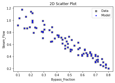
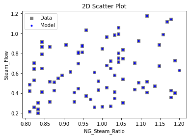
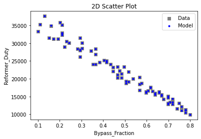
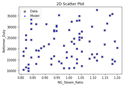
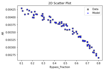
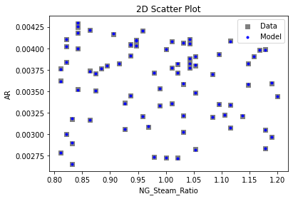
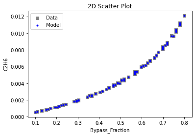
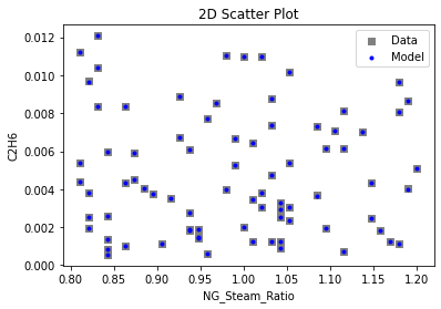
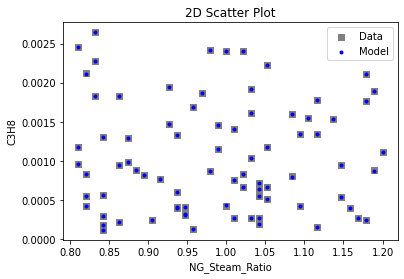
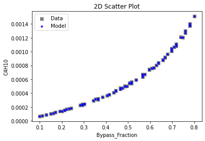
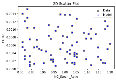
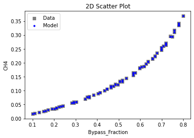
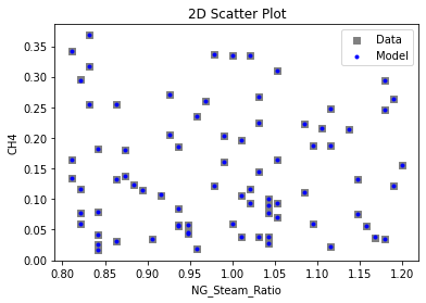
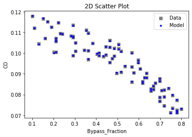
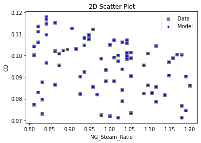
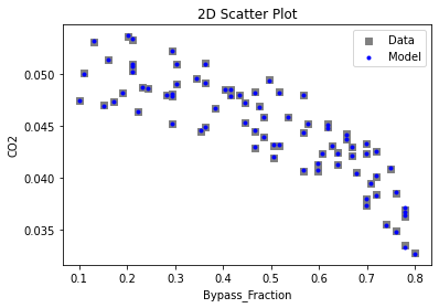
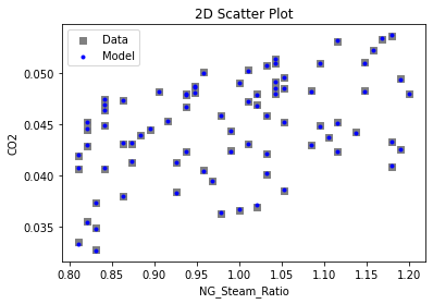
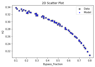
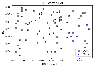
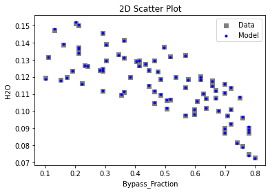
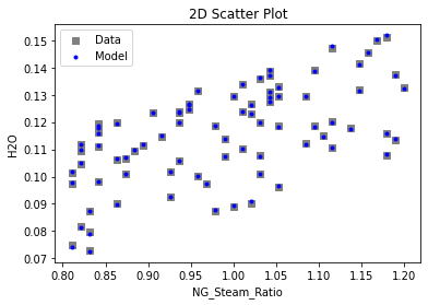
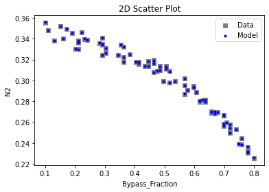
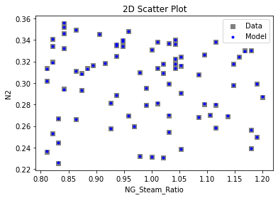
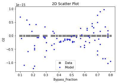
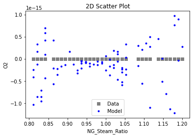
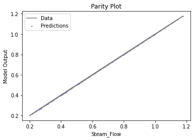
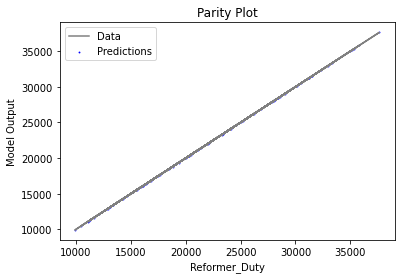
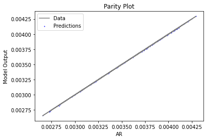
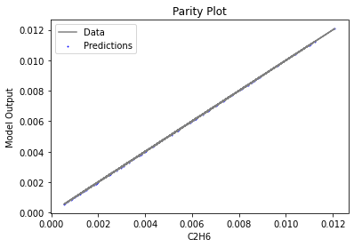
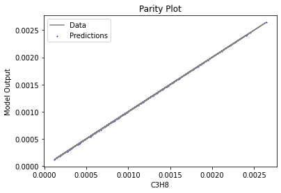
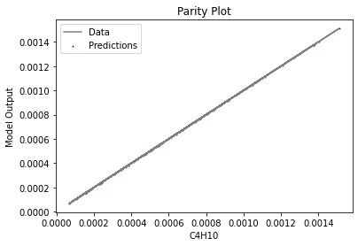
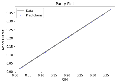
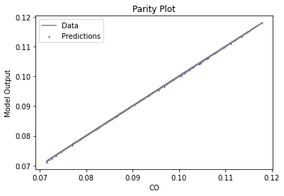
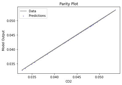
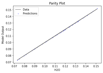
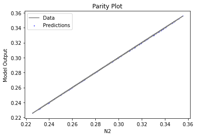
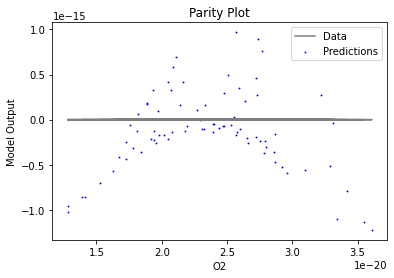
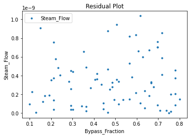
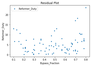
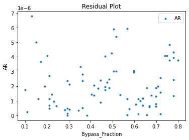
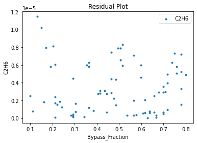
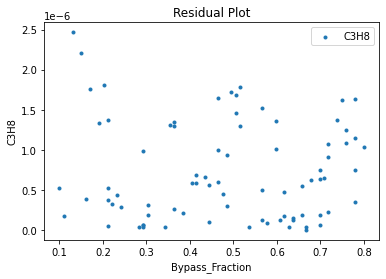
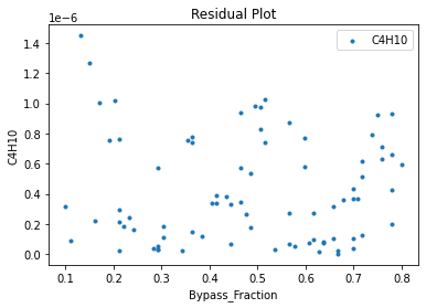
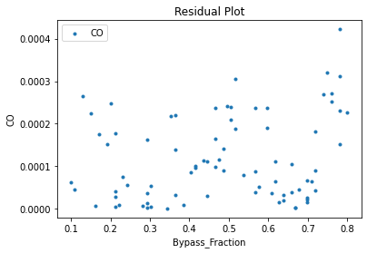
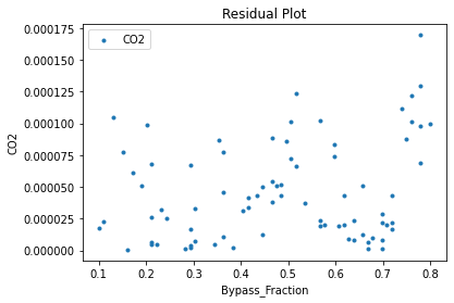
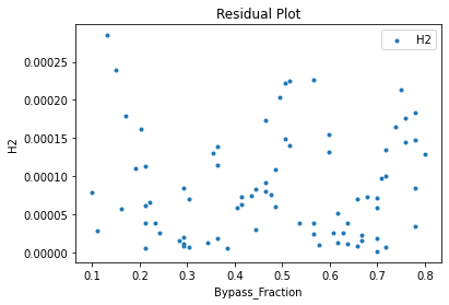
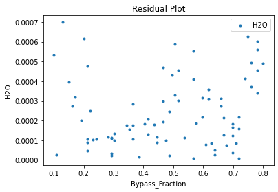
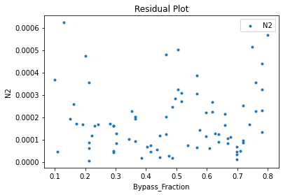
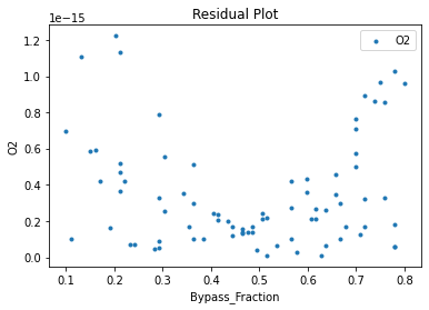
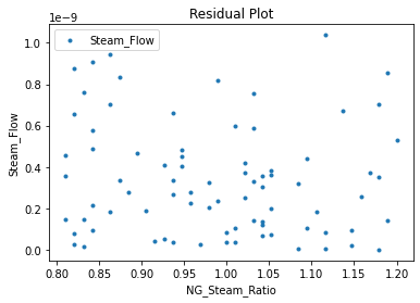
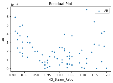
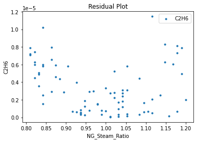
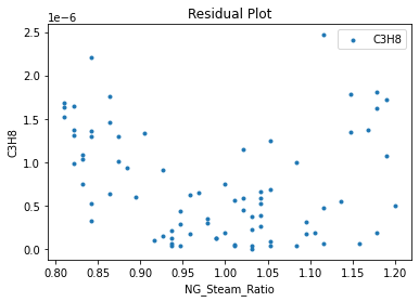
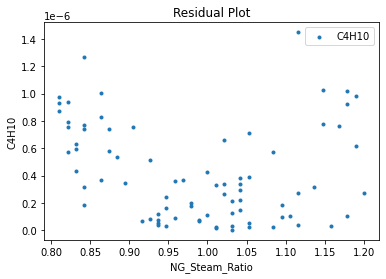
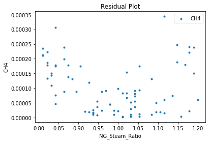
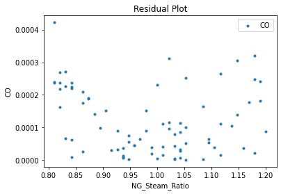
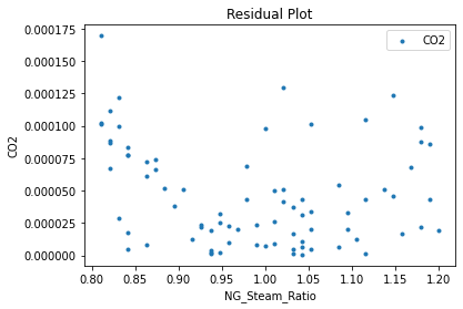
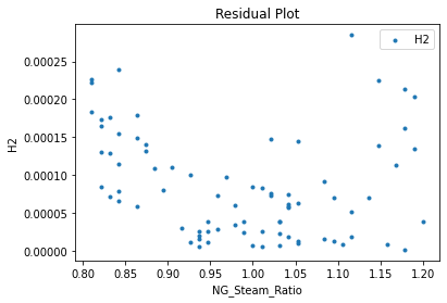
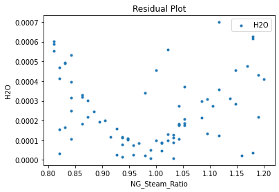
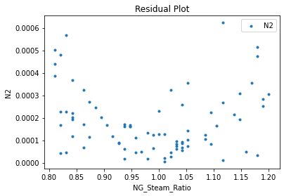
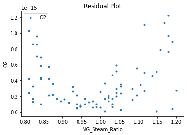
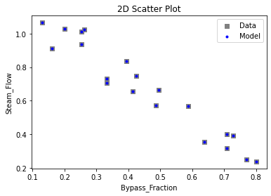
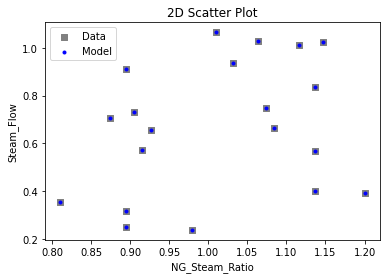
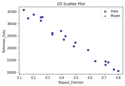
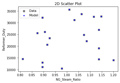
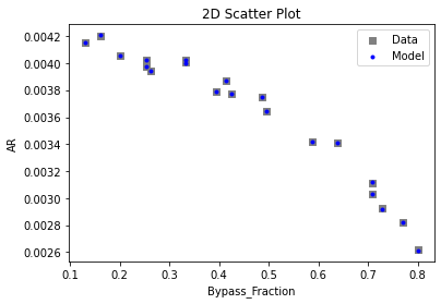
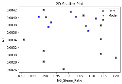
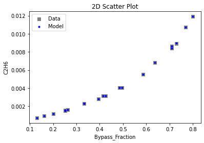
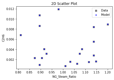
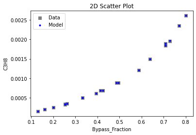
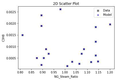
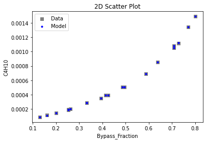
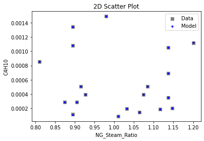
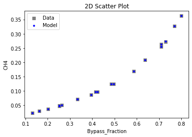
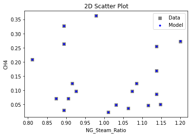
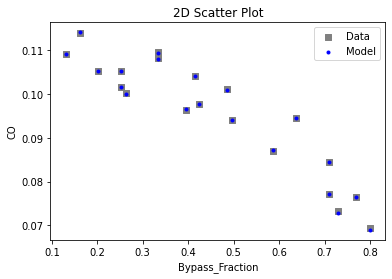
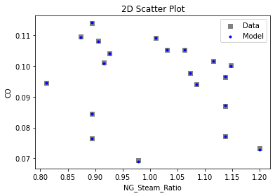
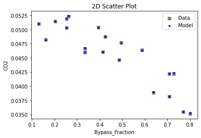
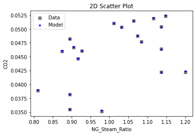
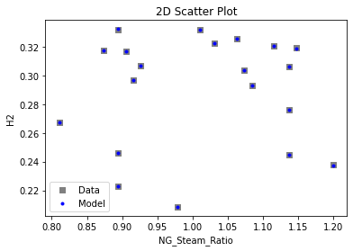
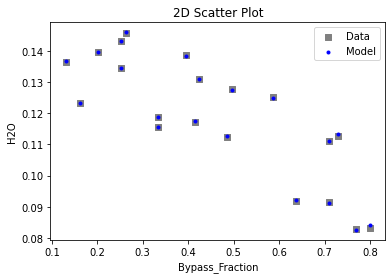
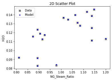
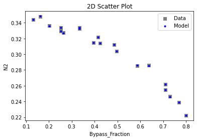
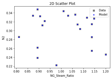
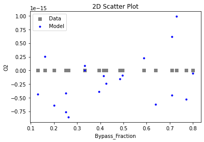
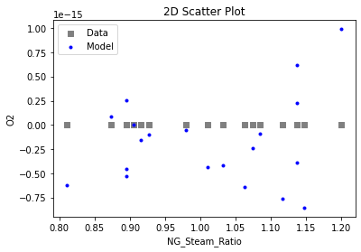
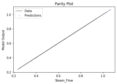
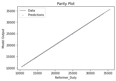
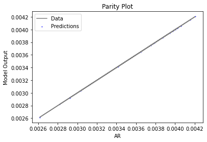
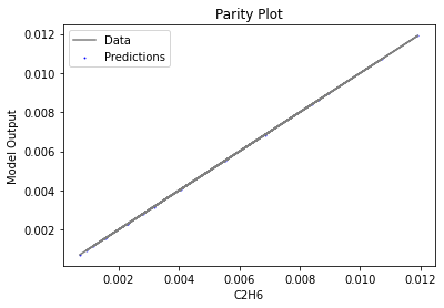
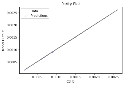
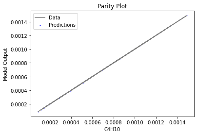
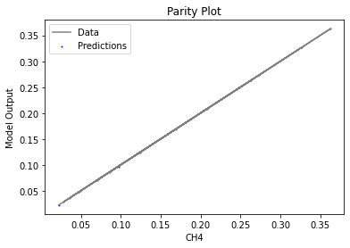
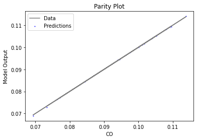
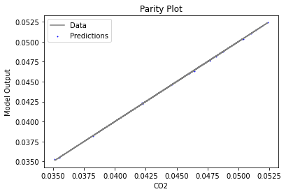
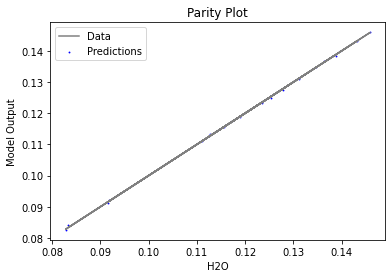
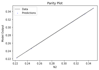
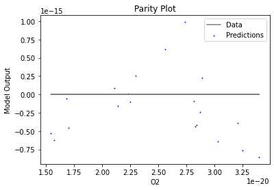
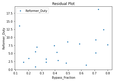
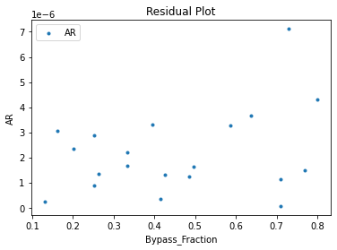
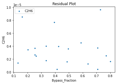
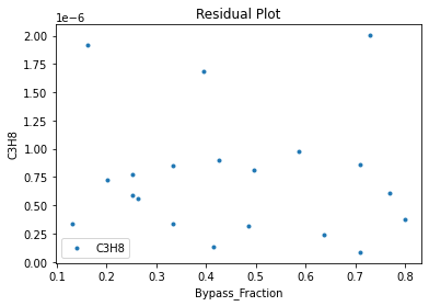
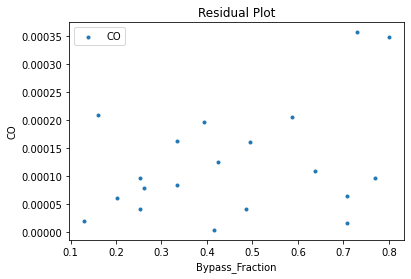
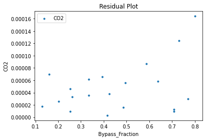
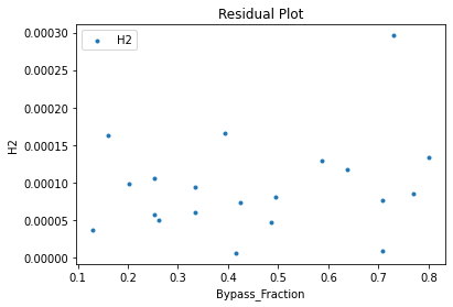
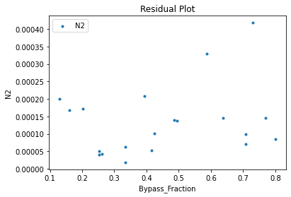
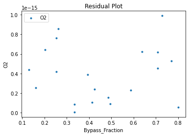
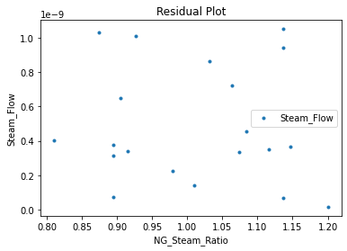
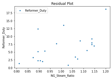
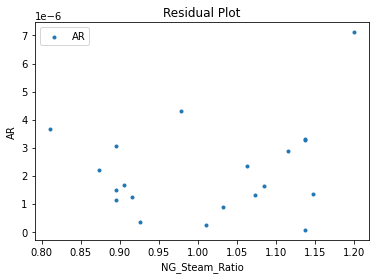
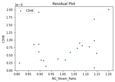
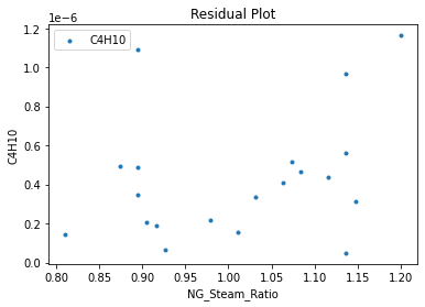
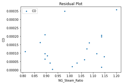
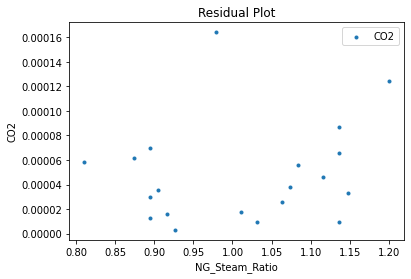
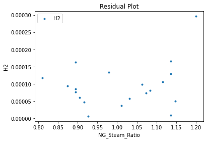
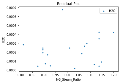
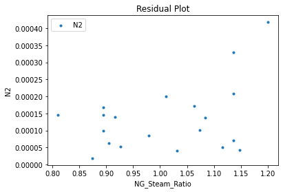
3.3 Visualizing surrogates

Now that the surrogate models have been trained, the models can be visualized through scatter, parity and residual plots to confirm their validity in the chosen domain. The training data will be visualized first to confirm the surrogates are fit the data, and then the validation data will be visualized to confirm the surrogates accurately predict new output values.

# visualize with IDAES surrogate plotting tools
surrogate_scatter2D(poly_surr, data_training, filename="pysmo_poly_train_scatter2D.pdf")
surrogate_parity(poly_surr, data_training, filename="pysmo_poly_train_parity.pdf")
surrogate_residual(poly_surr, data_training, filename="pysmo_poly_train_residual.pdf")

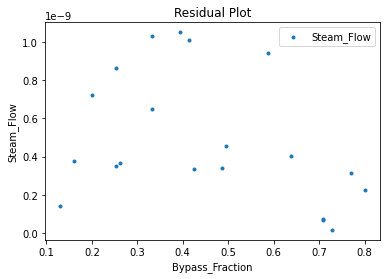
3.4 Model Validation

# visualize with IDAES surrogate plotting tools
surrogate_scatter2D(poly_surr, data_validation, filename="pysmo_poly_val_scatter2D.pdf")
surrogate_parity(poly_surr, data_validation, filename="pysmo_poly_val_parity.pdf")
surrogate_residual(poly_surr, data_validation, filename="pysmo_poly_val_residual.pdf")

4. IDAES Flowsheet Integration

4.1 Build and Run IDAES Flowsheet

Next, we will build an IDAES flowsheet and import the surrogate model object. Each output variable has a unique PySMO model expression, and the surrogate expressions may be added to the model via an indexed Constraint() component.

# create the IDAES model and flowsheet
m = ConcreteModel()
m.fs = FlowsheetBlock(dynamic=False)

# create flowsheet input variables
m.fs.bypass_frac = Var(
    initialize=0.80, bounds=[0.1, 0.8], doc="natural gas bypass fraction"
)
m.fs.ng_steam_ratio = Var(
    initialize=0.80, bounds=[0.8, 1.2], doc="natural gas to steam ratio"
)

# create flowsheet output variables
m.fs.steam_flowrate = Var(initialize=0.2, doc="steam flowrate")
m.fs.reformer_duty = Var(initialize=10000, doc="reformer heat duty")
m.fs.AR = Var(initialize=0, doc="AR fraction")
m.fs.C2H6 = Var(initialize=0, doc="C2H6 fraction")
m.fs.C3H8 = Var(initialize=0, doc="C3H8 fraction")
m.fs.C4H10 = Var(initialize=0, doc="C4H10 fraction")
m.fs.CH4 = Var(initialize=0, doc="CH4 fraction")
m.fs.CO = Var(initialize=0, doc="CO fraction")
m.fs.CO2 = Var(initialize=0, doc="CO2 fraction")
m.fs.H2 = Var(initialize=0, doc="H2 fraction")
m.fs.H2O = Var(initialize=0, doc="H2O fraction")
m.fs.N2 = Var(initialize=0, doc="N2 fraction")
m.fs.O2 = Var(initialize=0, doc="O2 fraction")

# create input and output variable object lists for flowsheet
inputs = [m.fs.bypass_frac, m.fs.ng_steam_ratio]
outputs = [
    m.fs.steam_flowrate,
    m.fs.reformer_duty,
    m.fs.AR,
    m.fs.C2H6,
    m.fs.C4H10,
    m.fs.C3H8,
    m.fs.CH4,
    m.fs.CO,
    m.fs.CO2,
    m.fs.H2,
    m.fs.H2O,
    m.fs.N2,
    m.fs.O2,
]

# create the Pyomo/IDAES block that corresponds to the surrogate
# PySMO

# capture long output (not required to use surrogate API)
stream = StringIO()
oldstdout = sys.stdout
sys.stdout = stream

surrogate = PysmoSurrogate.load_from_file("pysmo_poly_surrogate.json")
m.fs.surrogate = SurrogateBlock(concrete=True)
m.fs.surrogate.build_model(surrogate, input_vars=inputs, output_vars=outputs)

# revert back to normal output capture - don't need to print PySMO load output
sys.stdout = oldstdout

# fix input values and solve flowsheet
m.fs.bypass_frac.fix(0.5)
m.fs.ng_steam_ratio.fix(1)

solver = SolverFactory("ipopt")
status_obj, solved, iters, time, *_ = _run_ipopt_with_stats(m, solver)

2022-07-18 07:50:26 [INFO] idaes.core.surrogate.pysmo_surrogate: Decode surrogate. type=poly
Ipopt 3.13.2: output_file=C:\Users\BRANDO~1\AppData\Local\Temp\tmpdhc_oiziipopt_out
max_iter=500
max_cpu_time=120


******************************************************************************
This program contains Ipopt, a library for large-scale nonlinear optimization.
 Ipopt is released as open source code under the Eclipse Public License (EPL).
         For more information visit http://projects.coin-or.org/Ipopt

This version of Ipopt was compiled from source code available at
    https://github.com/IDAES/Ipopt as part of the Institute for the Design of
    Advanced Energy Systems Process Systems Engineering Framework (IDAES PSE
    Framework) Copyright (c) 2018-2019. See https://github.com/IDAES/idaes-pse.

This version of Ipopt was compiled using HSL, a collection of Fortran codes
    for large-scale scientific computation.  All technical papers, sales and
    publicity material resulting from use of the HSL codes within IPOPT must
    contain the following acknowledgement:
        HSL, a collection of Fortran codes for large-scale scientific
        computation. See http://www.hsl.rl.ac.uk.
******************************************************************************

This is Ipopt version 3.13.2, running with linear solver ma27.

Number of nonzeros in equality constraint Jacobian...:       13
Number of nonzeros in inequality constraint Jacobian.:        0
Number of nonzeros in Lagrangian Hessian.............:        0

Total number of variables............................:       13
                     variables with only lower bounds:        0
                variables with lower and upper bounds:        0
                     variables with only upper bounds:        0
Total number of equality constraints.................:       13
Total number of inequality constraints...............:        0
        inequality constraints with only lower bounds:        0
   inequality constraints with lower and upper bounds:        0
        inequality constraints with only upper bounds:        0

iter    objective    inf_pr   inf_du lg(mu)  ||d||  lg(rg) alpha_du alpha_pr  ls
   0  0.0000000e+00 1.11e+04 0.00e+00  -1.0 0.00e+00    -  0.00e+00 0.00e+00   0
   1  0.0000000e+00 0.00e+00 0.00e+00  -1.0 1.11e+04    -  1.00e+00 1.00e+00h  1

Number of Iterations....: 1

                                   (scaled)                 (unscaled)
Objective...............:   0.0000000000000000e+00    0.0000000000000000e+00
Dual infeasibility......:   0.0000000000000000e+00    0.0000000000000000e+00
Constraint violation....:   0.0000000000000000e+00    0.0000000000000000e+00
Complementarity.........:   0.0000000000000000e+00    0.0000000000000000e+00
Overall NLP error.......:   0.0000000000000000e+00    0.0000000000000000e+00


Number of objective function evaluations             = 2
Number of objective gradient evaluations             = 2
Number of equality constraint evaluations            = 2
Number of inequality constraint evaluations          = 0
Number of equality constraint Jacobian evaluations   = 2
Number of inequality constraint Jacobian evaluations = 0
Number of Lagrangian Hessian evaluations             = 1
Total CPU secs in IPOPT (w/o function evaluations)   =      0.002
Total CPU secs in NLP function evaluations           =      0.000

EXIT: Optimal Solution Found.

Let’s print some model results:

print("Model status: ", status_obj)
print("Solution optimal: ", solved)
print("IPOPT iterations: ", iters)
print("IPOPT runtime: ", time)

print()
print("Steam flowrate = ", value(m.fs.steam_flowrate))
print("Reformer duty = ", value(m.fs.reformer_duty))
print("Mole Fraction Ar = ", value(m.fs.AR))
print("Mole Fraction C2H6 = ", value(m.fs.C2H6))
print("Mole Fraction C3H8 = ", value(m.fs.C3H8))
print("Mole Fraction C4H10 = ", value(m.fs.C4H10))
print("Mole Fraction CH4 = ", value(m.fs.CH4))
print("Mole Fraction CO = ", value(m.fs.CO))
print("Mole Fraction CO2 = ", value(m.fs.CO2))
print("Mole Fraction H2 = ", value(m.fs.H2))
print("Mole Fraction H2O = ", value(m.fs.H2O))
print("Mole Fraction N2 = ", value(m.fs.N2))
print("Mole Fraction O2 = ", value(m.fs.O2))

Model status:  
Problem: 
- Lower bound: -inf
  Upper bound: inf
  Number of objectives: 1
  Number of constraints: 13
  Number of variables: 13
  Sense: unknown
Solver: 
- Status: ok
  Message: Ipopt 3.13.2\x3a Optimal Solution Found
  Termination condition: optimal
  Id: 0
  Error rc: 0
  Time: 0.21503710746765137
Solution: 
- number of solutions: 0
  number of solutions displayed: 0

Solution optimal:  True
IPOPT iterations:  1
IPOPT runtime:  0.002

Steam flowrate =  0.605930849905908
Reformer duty =  21072.18354404451
Mole Fraction Ar =  0.003681176332705635
Mole Fraction C2H6 =  0.004185619307363976
Mole Fraction C3H8 =  0.0005232226000381635
Mole Fraction C4H10 =  0.000915651933507209
Mole Fraction CH4 =  0.1278093376040153
Mole Fraction CO =  0.09704695423872685
Mole Fraction CO2 =  0.04598331382977046
Mole Fraction H2 =  0.29392801019518694
Mole Fraction H2O =  0.11955513634749963
Mole Fraction N2 =  0.30643113913639164
Mole Fraction O2 =  -1.249000902703301e-16

4.2 Optimizing the Autothermal Reformer

Extending this example, we will unfix the input variables and optimize hydrogen production. We will restrict nitrogen below 34 mol% of the product stream and leave all other variables unfixed.

Above, variable values are called in reference to actual objects names; however, as shown below this may be done much more compactly by calling the list objects we created earlier.

# unfix input values and add the objective/constraint to the model
m.fs.bypass_frac.unfix()
m.fs.ng_steam_ratio.unfix()
m.fs.obj = Objective(expr=m.fs.H2, sense=maximize)
m.fs.con = Constraint(expr=m.fs.N2 <= 0.34)

# solve the model
tmr = TicTocTimer()
status = solver.solve(m, tee=True)
solve_time = tmr.toc("solve")

# print and check results
assert abs(value(m.fs.H2) - 0.33) <= 0.01
assert value(m.fs.N2 <= 0.4 + 1e-8)
print("Model status: ", status)
print("Solve time: ", solve_time)
for var in inputs:
    print(var.name, ": ", value(var))
for var in outputs:
    print(var.name, ": ", value(var))

Ipopt 3.13.2: 

******************************************************************************
This program contains Ipopt, a library for large-scale nonlinear optimization.
 Ipopt is released as open source code under the Eclipse Public License (EPL).
         For more information visit http://projects.coin-or.org/Ipopt

This version of Ipopt was compiled from source code available at
    https://github.com/IDAES/Ipopt as part of the Institute for the Design of
    Advanced Energy Systems Process Systems Engineering Framework (IDAES PSE
    Framework) Copyright (c) 2018-2019. See https://github.com/IDAES/idaes-pse.

This version of Ipopt was compiled using HSL, a collection of Fortran codes
    for large-scale scientific computation.  All technical papers, sales and
    publicity material resulting from use of the HSL codes within IPOPT must
    contain the following acknowledgement:
        HSL, a collection of Fortran codes for large-scale scientific
        computation. See http://www.hsl.rl.ac.uk.
******************************************************************************

This is Ipopt version 3.13.2, running with linear solver ma27.

Number of nonzeros in equality constraint Jacobian...:       39
Number of nonzeros in inequality constraint Jacobian.:        1
Number of nonzeros in Lagrangian Hessian.............:        3

Total number of variables............................:       15
                     variables with only lower bounds:        0
                variables with lower and upper bounds:        2
                     variables with only upper bounds:        0
Total number of equality constraints.................:       13
Total number of inequality constraints...............:        1
        inequality constraints with only lower bounds:        0
   inequality constraints with lower and upper bounds:        0
        inequality constraints with only upper bounds:        1

iter    objective    inf_pr   inf_du lg(mu)  ||d||  lg(rg) alpha_du alpha_pr  ls
   0 -2.9392801e-01 2.33e-10 2.29e-02  -1.0 0.00e+00    -  0.00e+00 0.00e+00   0
   1 -2.9594434e-01 1.26e+00 1.83e-03  -1.7 4.91e+02    -  1.00e+00 1.00e+00f  1
   2 -3.1944078e-01 1.10e+02 9.95e-03  -2.5 5.87e+03    -  8.91e-01 1.00e+00h  1
   3 -3.2526940e-01 1.23e+02 5.84e-03  -2.5 4.84e+03    -  1.00e+00 1.00e+00h  1
   4 -3.2643490e-01 3.65e+01 6.21e-04  -2.5 2.31e+03    -  1.00e+00 1.00e+00h  1
   5 -3.2638212e-01 2.63e-02 1.43e-06  -2.5 1.43e+01    -  1.00e+00 1.00e+00h  1
   6 -3.3121488e-01 6.94e+01 9.33e-03  -3.8 3.79e+03    -  9.30e-01 1.00e+00h  1
   7 -3.3107389e-01 1.24e+00 1.07e-04  -3.8 2.23e+02    -  1.00e+00 1.00e+00h  1
   8 -3.3113833e-01 7.00e-03 1.90e-06  -3.8 3.90e+01    -  1.00e+00 1.00e+00h  1
   9 -3.3141911e-01 1.18e-01 8.89e-05  -5.7 2.33e+02    -  1.00e+00 1.00e+00h  1
iter    objective    inf_pr   inf_du lg(mu)  ||d||  lg(rg) alpha_du alpha_pr  ls
  10 -3.3142572e-01 4.23e-04 1.87e-07  -5.7 9.82e+00    -  1.00e+00 1.00e+00h  1
  11 -3.3142943e-01 2.49e-05 1.79e-08  -8.6 3.27e+00    -  1.00e+00 1.00e+00h  1
  12 -3.3142944e-01 3.49e-10 3.43e-13  -8.6 3.08e-03    -  1.00e+00 1.00e+00h  1

Number of Iterations....: 12

                                   (scaled)                 (unscaled)
Objective...............:  -3.3142943546624620e-01   -3.3142943546624620e-01
Dual infeasibility......:   3.4318533323761223e-13    3.4318533323761223e-13
Constraint violation....:   9.2763282987757224e-13    3.4924596548080444e-10
Complementarity.........:   2.5059064471148534e-09    2.5059064471148534e-09
Overall NLP error.......:   2.5059064471148534e-09    2.5059064471148534e-09


Number of objective function evaluations             = 13
Number of objective gradient evaluations             = 13
Number of equality constraint evaluations            = 13
Number of inequality constraint evaluations          = 13
Number of equality constraint Jacobian evaluations   = 13
Number of inequality constraint Jacobian evaluations = 13
Number of Lagrangian Hessian evaluations             = 12
Total CPU secs in IPOPT (w/o function evaluations)   =      0.008
Total CPU secs in NLP function evaluations           =      0.000

EXIT: Optimal Solution Found.
[+   0.25] solve
Model status:  
Problem: 
- Lower bound: -inf
  Upper bound: inf
  Number of objectives: 1
  Number of constraints: 14
  Number of variables: 15
  Sense: unknown
Solver: 
- Status: ok
  Message: Ipopt 3.13.2\x3a Optimal Solution Found
  Termination condition: optimal
  Id: 0
  Error rc: 0
  Time: 0.22667384147644043
Solution: 
- number of solutions: 0
  number of solutions displayed: 0

Solve time:  0.2452052000000151
fs.bypass_frac :  0.10000009180464237
fs.ng_steam_ratio :  1.1111834229471356
fs.steam_flowrate :  1.2119404450478533
fs.reformer_duty :  38820.99757562503
fs.AR :  0.004103160387430764
fs.C2H6 :  0.0005447148148714457
fs.C4H10 :  0.00011911847417089402
fs.C3H8 :  6.809341754672801e-05
fs.CH4 :  0.016971527468375807
fs.CO :  0.10486284211123467
fs.CO2 :  0.05348834219642045
fs.H2 :  0.3314294354662462
fs.H2O :  0.1484139338795353
fs.N2 :  0.3400000039706032
fs.O2 :  -1.1594487847385354e-15