###############################################################################
# The Institute for the Design of Advanced Energy Systems Integrated Platform
# Framework (IDAES IP) was produced under the DOE Institute for the
# Design of Advanced Energy Systems (IDAES).
#
# Copyright (c) 2018-2023 by the software owners: The Regents of the
# University of California, through Lawrence Berkeley National Laboratory,
# National Technology & Engineering Solutions of Sandia, LLC, Carnegie Mellon
# University, West Virginia University Research Corporation, et al.
# All rights reserved.  Please see the files COPYRIGHT.md and LICENSE.md
# for full copyright and license information.
###############################################################################

Flowsheet Gibbs Reactor Simulation and Optimization of Steam Methane Reforming#

Learning Outcomes#

Call and implement the IDAES GibbsReactor unit model
Construct a steady-state flowsheet using the IDAES unit model library
Connecting unit models in a flowsheet using Arcs
Fomulate and solve an optimization problem
- Defining an objective function
- Setting variable bounds
- Adding additional constraints

Problem Statement#

Following the previous example of Steam Methane Reformation in an Equilibrium Reactor, this example solves the flowsheet using a Gibbs Reactor instead. The steam methane reformation example is adapted from S.Z. Abbas, V. Dupont, T. Mahmud, Kinetics study and modelling of steam methane reforming process over a NiO/Al2O3 catalyst in an adiabatic packed bed reactor. Int. J. Hydrogen Energy, 42 (2017), pp. 2889-2903. Typically, the process follows the chemical equations below:

CH₄ + H₂O → CO + 3H₂
CO + H₂O → CO₂ + H₂

However, the GibbsReactor unit model solves the equilibrium by minimizing Gibbs free energy. Conveniently, this eliminates the need for a reaction package although a thermophysical package is still required.

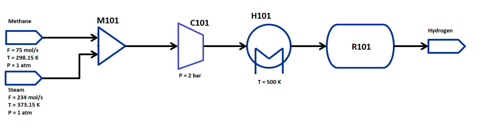
The flowsheet that we will be using for this module is shown below with the stream conditions. As in the prior example, we will be processing natural gas and steam feeds of fixed composition to produce hydrogen. The process consists of a mixer M101 for the two inlet streams, a compressor to compress the feed to the reaction pressure, a heater H101 to heat the feed to the reaction temperature, and a GibbsReactor unit R101. We will use thermophysical properties following the Peng-Robinsion cubic equation of state for this flowsheet.

The state variables chosen for the property package are total molar flows of each stream, temperature of each stream and pressure of each stream, and mole fractions of each component in each stream. The components considered are: CH₄, H₂O, CO, CO₂, and H₂ and the process occurs in vapor phase only. Therefore, every stream has 1 flow variable, 5 mole fraction variables, 1 temperature and 1 pressure variable.

Importing Required Pyomo and IDAES Components#

To construct a flowsheet, we will need several components from the Pyomo and IDAES packages, as well as some utility tools to build the flowsheet. For further details on these components, please refer to the Pyomo documentation.

From IDAES, we will be needing the FlowsheetBlock and the following unit models:

Feed
Mixer
Compressor
Heater
GibbsReactor
Product

from pyomo.environ import (
    Constraint,
    Var,
    ConcreteModel,
    Expression,
    Objective,
    TransformationFactory,
    value,
    units as pyunits,
)
from pyomo.network import Arc

from idaes.core import FlowsheetBlock
from idaes.models.properties.modular_properties import GenericParameterBlock
from idaes.models.unit_models import (
    Feed,
    Mixer,
    Compressor,
    Heater,
    GibbsReactor,
    Product,
)

from idaes_examples.mod.util import get_solver
from idaes.core.util.model_statistics import degrees_of_freedom
from idaes.core.util.initialization import propagate_state

Importing Required Thermophysical Package#

As mentioned earlier, the GibbsReactor does not require a reaction package.

Let us import the following module from the IDAES library:

natural_gas_PR as get_prop (method to get configuration dictionary)

from idaes.models_extra.power_generation.properties.natural_gas_PR import get_prop

Constructing the Flowsheet#

Let us create a ConcreteModel and add the flowsheet block.

m = ConcreteModel()
m.fs = FlowsheetBlock(dynamic=False)

We now need to add the property packages to the flowsheet. Unlike the previous example, we do not need to add a reaction package for the reactor model to calculate results. We will use the Modular Property Framework to build a state block for the parameter dictionary.

thermo_props_config_dict = get_prop(components=["CH4", "H2O", "H2", "CO", "CO2"])
m.fs.thermo_params = GenericParameterBlock(**thermo_props_config_dict)

Adding Unit Models#

Let us start adding the unit models we have imported to the flowsheet:

m.fs.CH4 = Feed(property_package=m.fs.thermo_params)
m.fs.H2O = Feed(property_package=m.fs.thermo_params)
m.fs.PROD = Product(property_package=m.fs.thermo_params)
m.fs.M101 = Mixer(
    property_package=m.fs.thermo_params, inlet_list=["methane_feed", "steam_feed"]
)
m.fs.H101 = Heater(
    property_package=m.fs.thermo_params,
    has_pressure_change=False,
    has_phase_equilibrium=False,
)
m.fs.C101 = Compressor(property_package=m.fs.thermo_params)

m.fs.R101 = GibbsReactor(
    property_package=m.fs.thermo_params,
    has_heat_transfer=True,
    has_pressure_change=False,
)

Connecting Unit Models Using Arcs#

We have now added all the unit models we need to the flowsheet. Let us connect the unit models by defining and building each Arc:

m.fs.s01 = Arc(source=m.fs.CH4.outlet, destination=m.fs.M101.methane_feed)
m.fs.s02 = Arc(source=m.fs.H2O.outlet, destination=m.fs.M101.steam_feed)
m.fs.s03 = Arc(source=m.fs.M101.outlet, destination=m.fs.C101.inlet)
m.fs.s04 = Arc(source=m.fs.C101.outlet, destination=m.fs.H101.inlet)
m.fs.s05 = Arc(source=m.fs.H101.outlet, destination=m.fs.R101.inlet)
m.fs.s06 = Arc(source=m.fs.R101.outlet, destination=m.fs.PROD.inlet)

Finally, we can use Pyomo’s TransformationFactory to write the equality constraints on each Arc:

TransformationFactory("network.expand_arcs").apply_to(m)

Adding Expressions to Compute Operating Costs#

For this flowsheet, we are interested in computing hydrogen production in millions of pounds per year, as well as the total costs due to pressurizing, cooling, and heating utilities:

Let us add Expressions to convert the product flow from mol/s to MM lb/year of hydrogen, and to calculate the cooling, heating and compression operating costs. The total operating cost will be the sum of the costs, expressed in \$/year assuming 8000 operating hours per year (~10% downtime, which is fairly common for small scale chemical plants):

m.fs.hyd_prod = Expression(
    expr=pyunits.convert(
        m.fs.PROD.inlet.flow_mol[0]
        * m.fs.PROD.inlet.mole_frac_comp[0, "H2"]
        * m.fs.thermo_params.H2.mw,  # MW defined in properties as kg/mol
        to_units=pyunits.Mlb / pyunits.yr,
    )
)  # converting kg/s to MM lb/year

m.fs.cooling_cost = Expression(
    expr=0.212e-7 * (m.fs.R101.heat_duty[0])
)  # the reaction is endothermic, so R101 duty is positive
m.fs.heating_cost = Expression(
    expr=2.2e-7 * m.fs.H101.heat_duty[0]
)  # the stream must be heated to T_rxn, so H101 duty is positive
m.fs.compression_cost = Expression(
    expr=0.12e-5 * m.fs.C101.work_isentropic[0]
)  # the stream must be pressurized, so the C101 work is positive
m.fs.operating_cost = Expression(
    expr=(3600 * 8000 * (m.fs.heating_cost + m.fs.cooling_cost + m.fs.compression_cost))
)

Fixing Feed Conditions#

We expect each stream to have 8 degrees of freedom, the mixer to have 0 (after both streams are accounted for), the compressor to have 2 (the pressure change and efficiency), the heater to have 1 (just the duty, since the inlet is also the outlet of M101), and the reactor to have 1 (conversion). Therefore, we have 20 degrees of freedom to specify: temperature, pressure, flow and mole fractions of all five components on both streams; compressor pressure change and efficiency; outlet heater temperature; and reactor conversion.

print(degrees_of_freedom(m))

Based on the literature source, we will initialize our simulation with the following values:

m.fs.CH4.outlet.mole_frac_comp[0, "CH4"].fix(1)
m.fs.CH4.outlet.mole_frac_comp[0, "H2O"].fix(1e-5)
m.fs.CH4.outlet.mole_frac_comp[0, "H2"].fix(1e-5)
m.fs.CH4.outlet.mole_frac_comp[0, "CO"].fix(1e-5)
m.fs.CH4.outlet.mole_frac_comp[0, "CO2"].fix(1e-5)
m.fs.CH4.outlet.flow_mol.fix(75 * pyunits.mol / pyunits.s)
m.fs.CH4.outlet.temperature.fix(298.15 * pyunits.K)
m.fs.CH4.outlet.pressure.fix(1e5 * pyunits.Pa)

m.fs.H2O.outlet.mole_frac_comp[0, "CH4"].fix(1e-5)
m.fs.H2O.outlet.mole_frac_comp[0, "H2O"].fix(1)
m.fs.H2O.outlet.mole_frac_comp[0, "H2"].fix(1e-5)
m.fs.H2O.outlet.mole_frac_comp[0, "CO"].fix(1e-5)
m.fs.H2O.outlet.mole_frac_comp[0, "CO2"].fix(1e-5)
m.fs.H2O.outlet.flow_mol.fix(234 * pyunits.mol / pyunits.s)
m.fs.H2O.outlet.temperature.fix(373.15 * pyunits.K)
m.fs.H2O.outlet.pressure.fix(1e5 * pyunits.Pa)

Fixing Unit Model Specifications#

For the initial problem, let us fix the compressor outlet pressure to 2 bar for now, the efficiency to 0.90 (a common assumption for compressor units), and the heater outlet temperature to 500 K. We will unfix these values later to optimize the flowsheet.

m.fs.C101.outlet.pressure.fix(pyunits.convert(2 * pyunits.bar, to_units=pyunits.Pa))
m.fs.C101.efficiency_isentropic.fix(0.90)
m.fs.H101.outlet.temperature.fix(500 * pyunits.K)

The GibbsReactor unit model calculates the amount of product and reactant based on the free energy minimization; therefore, we will specify a desired conversion and let the solver determine the reactor duty and heat transfer. For convenience, we will define the reactor conversion as the amount of methane that is converted.

m.fs.R101.conversion = Var(
    initialize=0.80, bounds=(0, 1), units=pyunits.dimensionless
)  # fraction

m.fs.R101.conv_constraint = Constraint(
    expr=m.fs.R101.conversion
    * m.fs.R101.inlet.flow_mol[0]
    * m.fs.R101.inlet.mole_frac_comp[0, "CH4"]
    == (
        m.fs.R101.inlet.flow_mol[0] * m.fs.R101.inlet.mole_frac_comp[0, "CH4"]
        - m.fs.R101.outlet.flow_mol[0] * m.fs.R101.outlet.mole_frac_comp[0, "CH4"]
    )
)

m.fs.R101.conversion.fix(0.80)

For initialization, we solve a square problem (degrees of freedom = 0). Let’s check the degrees of freedom below:

print(degrees_of_freedom(m))

Finally, we need to initialize the each unit operation and propagate the outlet results in sequence to solve the flowsheet:

# Initialize and solve each unit operation
m.fs.CH4.initialize()
propagate_state(arc=m.fs.s01)

m.fs.H2O.initialize()
propagate_state(arc=m.fs.s02)

m.fs.M101.initialize()
propagate_state(arc=m.fs.s03)

m.fs.C101.initialize()
propagate_state(arc=m.fs.s04)

m.fs.H101.initialize()
propagate_state(arc=m.fs.s05)

m.fs.R101.initialize()
propagate_state(arc=m.fs.s06)

m.fs.PROD.initialize()

# set solver
solver = get_solver()

# Solve the model
results = solver.solve(m, tee=True)

Analyze the Results of the Square Problem#

What is the total operating cost?

print(f"operating cost = ${value(m.fs.operating_cost)/1e6:0.3f} million per year")

For this operating cost, what conversion did we achieve of methane to hydrogen?

m.fs.R101.report()

print()
print(f"Conversion achieved = {value(m.fs.R101.conversion):.1%}")

Optimizing Hydrogen Production#

Now that the flowsheet has been squared and solved, we can run a small optimization problem to determine optimal conditions for producing hydrogen. Suppose we wish to find ideal conditions for the competing reactions. The GibbsReactor does not drive equilibrium forward based on temperature, so we will see small amounts of intermediate components present in the product stream. We will allow for variable reactor temperature and pressure by freeing our heater and compressor specifications, and minimize cost to achieve 90% methane conversion. Since we assume an isentopic compressor, allowing compression will heat our feed stream and reduce or eliminate the required heater duty.

Let us declare our objective function for this problem.

m.fs.objective = Objective(expr=m.fs.operating_cost)

Now, we need to add the design constraints and unfix the decision variables as we had solved a square problem until now, as well as set bounds for the design variables (reactor outlet temperature is set by state variable bounds in property package):

m.fs.R101.conversion.fix(0.90)

m.fs.C101.outlet.pressure.unfix()
m.fs.C101.outlet.pressure[0].setlb(
    pyunits.convert(1 * pyunits.bar, to_units=pyunits.Pa)
)  # equals inlet pressure
m.fs.C101.outlet.pressure[0].setlb(
    pyunits.convert(10 * pyunits.bar, to_units=pyunits.Pa)
)  # at most, pressurize to 1 bar

m.fs.H101.outlet.temperature.unfix()
m.fs.H101.heat_duty[0].setlb(
    0 * pyunits.J / pyunits.s
)  # ensures outlet is equal to or greater than inlet temperature
m.fs.H101.outlet.temperature[0].setub(1000 * pyunits.K)  # at most, heat to 1000 K

We have now defined the optimization problem and we are now ready to solve this problem.

results = solver.solve(m, tee=True)

print(f"operating cost = ${value(m.fs.operating_cost)/1e6:0.3f} million per year")

print()
print("Compressor results")

m.fs.C101.report()

print()
print("Heater results")

m.fs.H101.report()

print()
print("Gibbs reactor results")

m.fs.R101.report()

Display optimal values for the decision variables and design variables:

print("Optimal Values")
print()

print(f"C101 outlet pressure = {value(m.fs.C101.outlet.pressure[0])/1E6:0.3f} MPa")
print()

print(f"C101 outlet temperature = {value(m.fs.C101.outlet.temperature[0]):0.3f} K")
print()

print(f"H101 outlet temperature = {value(m.fs.H101.outlet.temperature[0]):0.3f} K")

print()
print(f"R101 outlet temperature = {value(m.fs.R101.outlet.temperature[0]):0.3f} K")

print()
print(f"Hydrogen produced = {value(m.fs.hyd_prod):0.3f} MM lb/year")

print()
print(f"Conversion achieved = {value(m.fs.R101.conversion):.1%}")

IDAES Examples

Flowsheet Gibbs Reactor Simulation and Optimization of Steam Methane Reforming

Contents